Selecting and Interpreting a Region for Analysis

Understanding the Australian Statistical Geography Standard (ASGS)

It is important to first have some understanding of the Australian Statistical Geography Standard (ASGS) structure.  The following descriptions are sourced from ABS Catalogue 1270.0.  Statistics provided by ABS are available at different levels, from mesh blocks that may contain less than three dwellings, through to Australia as a whole.  When the study is related to a rural locality or an urban suburb then the following are commonly used:

• Statistical Area Level 1 (SA1) – this is the smallest geographic area with disaggregated Census data available, and averages 400 usual residents.  It might not be big enough to adequately define a town or a suburb, but with its size comes versatility – SA1s can be easily combined to closely approximate most regions.
• Urban Centres and Localities (UCL) – this is defined by places that exhibit a cluster of people.  Its definition is based on density of the population and dwellings.
• Statistical Area Level 2 (SA2) – this is designed to represent a community, and varies in size from about 3,000 to 25,000 usual residents.  It is generally smaller in population in regional areas compared to urban centres.
• State Suburbs (SSC) – this is an approximation of localities gazetted by the Geographical Place Name authority for each State or Territory.  It conforms well to both urban suburbs and rural localities.
• Local Government Areas (LGA) – this is an ABS approximation of officially gazetted Local Government Areas.  In urban centres, it is usually an approximate grouping of suburbs, whereas in rural localities it usually includes one or more large towns, plus the outlying areas in between. 

Examples - Defining a Target Population and Catchment Area

The following examples demonstrate how Data Analysis Australia can tailor the selection of regions and data depending on the situation.  Two types of locality will be considered: a rural town (Karratha) and an urban suburb (Baldivis), and four types of geographic boundaries.

• Karratha is a town in the Pilbara region of Western Australia which has been developed over time to accommodate a growing workforce from the Resources Industry, with a number of mining sites in the surrounding areas.  
• Baldivis is a developing residential suburb located in the southern outskirts of the Perth Metropolitan area.  This area consists of mostly residential estates, with a higher than State average proportion of separate houses, as opposed to apartments, etcetera, and a relatively higher number of family households.

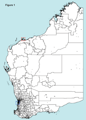
Figure 1 demonstrates the localities of Karratha (red dashed box) and Baldivis (blue dashed box) in the context of the State as a whole.  The black boundary lines represent SA1s.

Example 1 - Statistical Area Level 1 (SA1) 

The advantage of using SA1s is their flexibility.  It is the smallest unit area for which disaggregated Census data is available, and hence is the go-to geography for when a well-defined region needs to be replicated using the ASGS, or if one of the larger geographical areas is not quite right.  If a circular catchment area was defined as distance from a particular point, then a selection of SA1s would get you the closest match to your catchment area.  Examples of where this approach may be applied are for market research, liquor licensing applications, identifying potential fire danger areas (environmental effects aside), or replicating enrolment boundaries for schools.

The higher level ASGS regions can be built up from SA1s, so you may well ask why not always use SA1s as your base unit?  First, if one of the higher level ASGS regions is precisely relevant for your needs, then there’s no reason to complicate matters.  It is not always as simple as adding together data for each SA1, as statistics such as medians and socio-economic indexes need more particular consideration.  Secondly, a general rule is that the finer the level of the geography, the less data is available.  For example, the working population profile – based on location of employment – is not released by the ABS at SA1 level.  If this was critical to your analysis, then using SA1s to define your area would be fundamentally flawed.

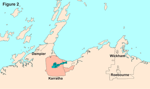
Figure 2 shows a selection of SA1s around the town centre of Karratha in green, with less densely populated areas of the town in orange, and other SA1 boundaries shown via black lines.  It may be useful to analyse the two subsets of the town of Karratha to inform a potential residential housing development project, and the use of SA1s makes this possible.  As you can see, the SA1s are smaller in the more populated areas, and larger in the less populated areas.  Other clusters of smaller, more densely populated SA1s are identifiable in Figure 2.  These represent the localities of Dampier, to the North-West of Karratha, and Wickham and Roebourne to the East. 

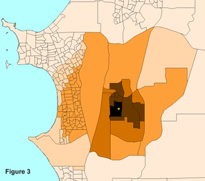
Figure 3 shows a selection of SA1s surrounding a randomly selected point within Baldivis.  It can be seen that the more established areas along the coastline are represented by smaller, more densely populated SA1s, whereas the SA1s in the developing area of Baldivis are larger and more sparsely populated.  A selection of SA1s like that presented here may be appropriate when analysing the patronage of a particular business, with shades representing frequency or average size of purchases for weighting purposes. 

Example 2 - Urban Centres/Localities (UCL)

Urban Centres or Localities are defined by a combination of SA1s consisting of a relatively densely populated centre, with surrounding SA1s that could reasonably be associated with that centre.  The use of a UCL, rather than the selection of SA1s that defines it, is an appropriate area for analysis in many instances, and its use can simplify issues relating to producing combined statistics, such as medians, that involve more than simply summing data. 

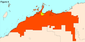
In regional and rural Western Australia particularly, a UCL can quite neatly and simply define a city or town.  The UCL is helpful in defining regional town centres, when outlying areas are not of interest.  If the highlighted SA1s for Karratha from Figure 2 are combined, this defines the Karratha UCL.  At the regional level, moving from a UCL level up to a Local Government Area level can result in a significant increase in area, see Figure 4 demonstrating the Karratha UCL (in yellow) within the Shire of Roebourne LGA (orange).  In the example of Karratha, the SA2 actually defines the same area as the UCL.  This is an important feature to recognise, as additional statistics are available at the SA2 level (that are not available at the UCL level).  The path taken in sourcing data can lead to the belief that information is not available, when this may not be the case.  

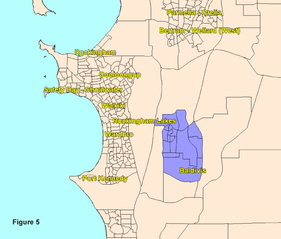
Within the Perth metropolitan area, UCLs can neatly define communities, but they are generally closer to and more accessible from neighbouring UCLs than in the regional situation.  Therefore a catchment area in the Perth metropolitan area is likely to include parts of surrounding communities, rather than the UCL alone.  Figure 5 shows the UCL of Baldivis (highlighted in purple).  It appears to define this community fairly well.  However, the suburbs of Warnbro, Port Kennedy, Waikiki etcetera are sufficiently close that one would expect some crossover with these suburbs for a business catchment area or other analytical interest. 

Example 3 - Statistical Area Level 2 (SA2)

The SA2s are designed to represent a community.  In the regional context this can define a smaller area than a UCL (e.g. for larger cities such as Geraldton or Kalgoorlie), an identical area to a UCL (e.g. Karratha as discussed previously), or a larger area that may include both a significant part of the UCL as well as some outlying areas (e.g. Esperance).  In the Perth metropolitan area, an SA2 can be roughly considered as a greater suburb, or grouping of suburbs.  A significant difference between SA2s and UCLs is that UCLs define “pockets” of areas, whereas SA2s fit together, like pieces of a jigsaw puzzle, to make up Western Australia and even Australia as a whole.  

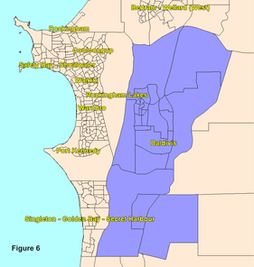
Another issue that needs consideration is that changes in the boundaries of ABS geographic areas can occur from time to time.  As seen in Figure 6, the Baldivis SA2 includes a significant stretch of land along the central southern corridor of the Perth metropolitan area.  This is an area with a number of residential estates established since the 2011 Census, and population growth and an increase in density in this area could well cause the definition of this community to change.  If it can be identified that an area may be particularly subject to a change in definition, and ongoing time series analysis is on the agenda, it is important to recognise this potential difficulty.

Example 4 - Local Government Area (LGA)

The Local Government Areas are a non-ABS structure.  As an administrative area, the region they define can group together areas that otherwise may not be sensical to do so, or may draw boundaries directly through neighbourhoods.  Due to their political nature, they are also quite subject to change.  While clearly it is a useful area for analysis relating to Local Government operations, there are also many planning decisions based on these boundaries.  It is important to note the similar geographic region of a Statistical Local Area (SLA) at this point.  In Western Australia, this is typically identical to the Local Government Area, with some exceptions such as the LGA of Harvey, which is split into the SLA of Harvey Part A, and Harvey Part B.

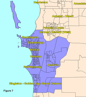
The LGA of the Shire of Roebourne (which contains Karratha) was presented in Figure 4.  It is typical for a regional LGA in Western Australia to include one or more towns that are reasonably close-by, plus outlying areas.  In the Perth Metropolitan area, it is an administrative grouping of suburbs or parts of suburbs.  Baldivis is located within the City of Rockingham, which is highlighted in purple in Figure 7.  Its 2011 Census count of usual residents is over 100,000 people, making it the sixth largest LGA in Western Australia (behind the Cities of Stirling, Joondalup, Wanneroo, Swan and Gosnells).  Due to its size, it is likely to contain communities that are highly different in nature.  Therefore, it may be desirable to analyse different subsets of the LGA (which may be approximated using SA1s, SA2s or combinations thereof) to ensure this variability is captured.

Further Information 

The examples and regions discussed in this Analytical Idea are by no means a complete review of the considerations involved when defining areas for analysis.  However, they do provide some insight into the nature of the ASGS regions, and highlight the value of statistical know-how and Census data experience in ensuring the analytical approach is fit-for-purpose. 

Data Analysis Australia recognises that while questions posed by different clients might seem similar, the required approach could be vastly different.  To ensure that clients’ queries are answered in the most relevant manner, Data Analysis Australia considers each enquiry on a case by case basis in order to establish the ‘best’ answer for the aim of the study.  The extensive experience accumulated from previous studies and the in-depth knowledge Data Analysis Australia exhibits regarding Census data ensures requests from clients can be responded to in a fit-for-purpose, strategic manner.  

Please Contact Us if you wish to discuss your demographic profiling needs with a Consultant Statistician.

March 2013